from datetime import datetime, timedelta
import os
import subprocess
import tempfile
from typing import Union
import contextily as ctx
import folium
import geopandas as gpd
from haversine import haversine, Unit
import matplotlib.pyplot as plt
import pandas as pd
import pydeck as pdk
import pyproj
import r5py
import requests
from sklearn import preprocessing
from shapely.geometry import LineString, Point, PolygonBicycle Network Modelling with r5py
Tutorial
Transport Modelling
REST API
Web data
Geospatial
r5py
pydeck
Analysing service coverage in London’s Santander Bike network.
Introduction
r5py is a relatively new transport modelling package available on PyPI. It provides convenient wrappers to Conveyal’s r5 Java library, a performant routing engine originating from the ubiquitous Open Trip Planner (OTP). Whereas r5py may not be as feature-rich as OTP, its unique strength is in the production of origin:destination matrices at scale. This is important if the intention is to produce stable statistics based on routing algorithms, where the idiosyncrasies of local transport service availability means that departure times can have a significant impact upon overall journey duration.
r5py achieves stable statistics by calculating travel times over multiple journeys within a time window, returning summaries such as the median travel time from point A to B.
A Note on the Purpose
This tutorial aims to familiarise the reader with r5py and how it integrates with the python geospatial ecosystem of packages. This article is not to be used to attempt to infer service quality outcomes. Limitations of this analysis and suggested improvements will be discussed throughout.
Intended Audience
Experienced python practitioners with a robust working knowledge of the typical python GIS stack, eg geopandas, shapely and folium and coordinate reference systems (CRS). Familiarity with r5py is not assumed.
Outcomes
- Ingest London bike charging station locations.
- Visualise charging stations in an interactive hex map.
- Generate a naive point plane of destinations.
- Check that the point plane is large enough to accommodate station locations.
- Adjust point plane locations to ensure routability.
- Calculate origin:destination travel time matrix, by cycling modality and with a maximum journey time of 30 minutes.
- Engineer features to help analyse the cycling network accessibility.
- Visualise the cycling network coverage and the most remote points within that area.
What You’ll Need:
requirements.txt
contextily
geopandas
haversine
folium
mapclassify
matplotlib
pydeck
pyproj
r5py
requests
scikit-learn
Configuring Java
It is required to configure a Java Virtual Machine for this tutorial. The transport routing depends on this. Please consult the r5py installation documentation [1] for guidance. In order to check that you have a compatible Java environment, run r5py.TransportNetwork(osm_pth) after exercise 1. For reference, I have used OpenJDK to manage my Java instance:
openjdk 11.0.19 2023-04-18 LTS
OpenJDK Runtime Environment Corretto-11.0.19.7.1 (build 11.0.19+7-LTS)
OpenJDK 64-Bit Server VM Corretto-11.0.19.7.1 (build 11.0.19+7-LTS, mixed mode)
London Cycle Station Service Coverage
Start by loading the required packages.
Street Network Data
Firstly, we must acquire information about the transport network. There are a few sources of this, but we shall use the BBBikes website to ingest London-specific OpenStreetMap extracts. The required data should be in protocol buffer (.pbf) format.
Exercise 1
Find the appropriate url that points to the london.osm.pbf file. Ingest the data and store at an appropriate location.
Click to expand hint
Either using python requests or subprocess with the curl command, request the url of the pbf file and output the response to a data folder.
Solution
Show the code
# As the osm files are large, I will use a tmp directory, though feel free to
# store the data wherever you like.
tmp = tempfile.TemporaryDirectory()
osm_pth = os.path.join(tmp.name, "london.osm.pbf")
subprocess.run(
    [
        "curl",
        "https://download.bbbike.org/osm/bbbike/London/London.osm.pbf",
        "-o",
        osm_pth,
    ]
)
% Total % Received % Xferd Average Speed Time Time Time Current
Dload Upload Total Spent Left Speed
0 0 0 0 0 0 0 0 --:--:-- --:--:-- --:--:-- 0 0 0 0 0 0 0 0 0 --:--:-- --:--:-- --:--:-- 0 45 103M 45 47.4M 0 0 43.0M 0 0:00:02 0:00:01 0:00:01 43.0M100 103M 100 103M 0 0 49.8M 0 0:00:02 0:00:02 --:--:-- 49.8MCompletedProcess(args=['curl', 'https://download.bbbike.org/osm/bbbike/London/London.osm.pbf', '-o', '/var/folders/qc/rrswmfbx1_v0sxklq1kr28jw0000gp/T/tmprnd4etkn/london.osm.pbf'], returncode=0)Bike Charging Station Locations
Exercise 2
To get data about the bike charging stations in London, we will query Transport for London’s BikePoint API.
- Explore the site and find the correct endpoint to query.
- The tutorial requires the following fields: station ID, the human-readable name, latitude and longitude for each available station.
- Store the data in a
geopandasgeodataframe with the appropriate coordinate reference system. - Inspect the head of the geodataframe.
Click to expand hint
- Using the requests package, send a get request to the endpoint.
- Store the required fields in a list: “id”, “commonName”, “lat”, “lon”.
- Check that the response returned HTTP status 200. If True, get the content in JSON format.
- Create an empty list to store the station data.
- Iterate through the content dictionaries. If a key is present within the required fields, store the key and value within a temporary dictionary.
- Append the dictionary of required fields and their values to the list of stations.
- Convert the list of dictionaries to a pandas dataframe. Then convert this to a
geopandasgeodataframe, using the coordinate reference system “EPSG:4326”. As we have lat and lon in separate columns, usegeopandaspoints_from_xy(), ensuring you pass values in the order of longitude, latitude. - Print out the head of the stations gdf.
Solution
Show the code
ENDPOINT = "https://api.tfl.gov.uk/BikePoint/"
resp = requests.get(ENDPOINT)
if resp.ok:
    content = resp.json()
else:
    raise requests.exceptions.HTTPError(
        f"{resp.status_code}: {resp.reason}"
    )

needed_keys = ["id", "commonName", "lat", "lon"]
all_stations = list()
for i in content:
    node_dict = dict()
    for k, v in i.items():
        if k in needed_keys:
            node_dict[k] = v
    all_stations.append(node_dict)

stations = pd.DataFrame(all_stations)
station_gdf = gpd.GeoDataFrame(
    stations,
    geometry=gpd.points_from_xy(stations["lon"], stations["lat"]),
    crs=4326,
)

station_gdf.head()| id | commonName | lat | lon | geometry | |
|---|---|---|---|---|---|
| 0 | BikePoints_1 | River Street , Clerkenwell | 51.529163 | -0.109970 | POINT (-0.10997 51.52916) |
| 1 | BikePoints_2 | Phillimore Gardens, Kensington | 51.499606 | -0.197574 | POINT (-0.19757 51.49961) |
| 2 | BikePoints_3 | Christopher Street, Liverpool Street | 51.521283 | -0.084605 | POINT (-0.08460 51.52128) |
| 3 | BikePoints_4 | St. Chad's Street, King's Cross | 51.530059 | -0.120973 | POINT (-0.12097 51.53006) |
| 4 | BikePoints_5 | Sedding Street, Sloane Square | 51.493130 | -0.156876 | POINT (-0.15688 51.49313) |
That’s all the external data needed for this tutorial. Let’s now examine the station locations.
Station Density
As the stations are densely located in and around central London, a standard matplotlib point map would suffer from overplotting. A better way is to present some aggregated value on a map, such as density.
Exercise 3
Plot the density of cycle station locations on a map. The solution will use pydeck, but any visualisation library that can handle geospatial data would be fine.
Click to expand hint
- Create a pydeck hexagon layer based on the
station_gdf. The hexagon layer should be configured as below:
- extruded
- position from lon and lat columns
- elevation scale is 100
- elevation range from 0 through 100
- coverage is 1
- radius of hexagons is 250 metres
- Create a pydeck view state object to control the initial position of the camera. Configure this as you see fit.
- (Optional) Add a custom tooltip, clarifying that the hexagon elevation is equal to the count of stations within that area. You may wish to consult the deck.gl documentation to help implement this.
- Create a deck with the hexagon layer, custom view state, tooltip and a map style of your choosing.
Solution
Show the code
# pydeck visuals - concentration of charging stations by r250m hex
layer = pdk.Layer(
    "HexagonLayer",
    station_gdf,
    pickable=True,
    extruded=True,
    get_position=["lon", "lat"],
    auto_highlight=True,
    elevation_scale=100,
    elevation_range=[0, 100],
    coverage=1,
    radius=250,  # in metres, default is 1km
    colorRange=[
        [255, 255, 178, 130],
        [254, 217, 118, 130],
        [254, 178, 76, 130],
        [253, 141, 60, 130],
        [240, 59, 32, 130],
        [189, 0, 38, 130],
    ], # optionally added rgba values to allow transparency
)
view_state = pdk.ViewState(
    # longitude=-0.140,# value for iframe
    longitude=-0.070,# value for code chunk
    latitude=51.535,
    # zoom=10, # value for iframe
    zoom=10.5, # value for code chunk
    min_zoom=5,
    max_zoom=15,
    pitch=40.5,
    bearing=-27.36,
)
tooltip = {"html": "<b>n Stations:</b> {elevationValue}"}
r = pdk.Deck(
    layers=[layer],
    initial_view_state=view_state,
    tooltip=tooltip, # prettier than default tooltip
    map_style=pdk.map_styles.LIGHT,
)
r
Generate Destinations
We can use the bike stations as journey origins. To compute travel times, we need to generate destination locations. This tutorial uses a simple approach to generating equally spaced points within a user-defined bounding box.
Limitation
Generating a point plane is a fast way to get a travel time matrix. However, this is naive to locations that the riders would prefer to start or finish their journeys. A more robust approach would be to use locations of retail or residential features. The European Commission’s Global Human Settlement Layer [2] data would provide centroids to every populated grid cell down to a 10m2 resolution.
Exercise 4
Write a function called create_point_grid() that will take the following parameters:
bbox_listexpecting a bounding box list in [xmin, ymin, xmax, ymax] format with epsg:4326 longitude & latitude values.stepsizeexpecting a positive integer, specifying the spacing of the grid points in metres.
create_point_grid() should return a geopandas geodataframe of equally spaced point locations - the point grid. The grid point locations should be in epsg:4326 projection. The geodataframe requires a geometry column and an id column equal to the index of the dataframe (required for r5py origin:destination matrix calculation).
Once you are happy with the function, use it to produce an example geodataframe and explore() a folium map of the point grid.
Click to expand hint
Note that epsg:4326 is a geodetic projection, unsuitable for measuring distance between points in the point plane. Ensure that the crs is re-projected to an appropriate planar crs for distance calculation.
- Store the South-West and North-East coordinates as
shapely.geometry.Pointobjects. - Use
pyproj.Transformer.from_crs()to create 2 transformers, one from geodetic to planar, and the other back from planar to geodetic. - Use the transformers to convert the SW and NE points from geodetic to planar.
- Use nested loops to iterate over the area between the corner points. Store the point location as a
shapely.geometry.Pointobject. Append the point to a list of grid points. - Increment the x and y values by the provided
stepsizeand continue to append points in this fashion until xmin has reached the xmax value and ymin has met the ymax value. - Ensure the stored coordinates are converted back to epsg:4326.
- Create a pandas dataframe with the geometry column using the appended point locations and an
idcolumn that uses therange()function to generate a unique integer value for each row. - Use the defined function with a sample bounding box and explore the resulting geodataframe with an interactive
foliummap.
Solution
Show the code
def create_point_grid(bbox_list: list, stepsize: int) -> gpd.GeoDataFrame:
    """Create a metric point plane for a given bounding box.

    Return a geodataframe of evenly spaced points for a specified bounding box.
    Distance between points is controlled by stepsize in metres.  As
    an intermediate step requires transformation to epsg:27700, the calculation
    of points is suitable for GB only.

    Parameters
    ----------
    bbox_list : list
        A list in xmin, ymin, xmax, ymax order. Expected to be in epsg:4326.
        Use https://boundingbox.klokantech.com/ or similar to export a bbox.
    stepsize : int
        Spacing of grid points in metres. Must be larger than zero.

    Returns
    -------
    gpd.GeoDataFrame
        GeoDataFrame in epsg:4326 of the point locations.

    Raises
    ------
    TypeError
        bbox_list is not type list.
        Coordinates in bbox_list are not type float.
        step_size is not type int.
    ValueError
        bbox_list is not length 4.
        xmin is greater than or equal to xmax.
        ymin is greater than or equal to ymax.
        step_size is not a positive integer.

    """
    # defensive checks
    if not isinstance(bbox_list, list):
        raise TypeError(f"bbox_list expects a list. Found {type(bbox_list)}")
    if not len(bbox_list) == 4:
        raise ValueError(f"bbox_list expects 4 values. Found {len(bbox_list)}")
    for coord in bbox_list:
        if not isinstance(coord, float):
            raise TypeError(
                f"Coords must be float. Found {coord}: {type(coord)}"
            )
    # check points are ordered correctly
    xmin, ymin, xmax, ymax = bbox_list
    if xmin >= xmax:
        raise ValueError(
            "bbox_list value at pos 0 should be smaller than value at pos 2."
        )
    if ymin >= ymax:
        raise ValueError(
            "bbox_list value at pos 1 should be smaller than value at pos 3."
        )
    if not isinstance(stepsize, int):
        raise TypeError(f"stepsize expects int. Found {type(stepsize)}")
    if stepsize <= 0:
        raise ValueError("stepsize must be a positive integer.")

    # Set up crs transformers. Need a planar crs for work in metres - use BNG
    planar_transformer = pyproj.Transformer.from_crs(4326, 27700)
    geodetic_transformer = pyproj.Transformer.from_crs(27700, 4326)
    # bbox corners
    sw = Point((xmin, ymin))
    ne = Point((xmax, ymax))
    # Project corners to planar
    planar_sw = planar_transformer.transform(sw.x, sw.y)
    planar_ne = planar_transformer.transform(ne.x, ne.y)
    # Iterate over metric plane
    points = []
    x = planar_sw[0]
    while x < planar_ne[0]:
        y = planar_sw[1]
        while y < planar_ne[1]:
            p = Point(geodetic_transformer.transform(x, y))
            points.append(p)
            y += stepsize
        x += stepsize
    df = pd.DataFrame({"geometry": points, "id": range(0, len(points))})
    gdf = gpd.GeoDataFrame(df, crs=4326)
    return gdf

create_point_grid(
  bbox_list=[-0.5917,51.2086,0.367,51.7575], stepsize=5000).explore(min_zoom=9)
Make this Notebook Trusted to load map: File -> Trust Notebook
Study Area Size
Before we go ahead with the transport modelling, it is important to check that the point plane is large enough to contain a 30 minute journey from any of the stations. 30 minutes is the current charging interval for the pay as you ride options [3]. Note that making the point plane larger or the step size smaller means more travel times to calculate, so there is a compromise to be met. Using too small a grid will introduce edge effects [4] and therefore limit the validity of the study.
Exercise 5
Check that the point plane study area is large enough to accommodate an estimation of reachable area from the station locations.
Part 1
- Create a
point_planeobject withcreate_point_grid()that has a bounding box of your choosing. Use a stepsize of 1000 metres. - Get the boundary polygon of this point plane. This is the study area.
- Buffer the bike station locations. This buffered area should represent the reachable area from within a 30 minute ride of any station and a presumed average urban cycle speed of 18 kilometres per hour (an opinionated speed based on a sample of one overweight, middle-aged man’s Strava data). Store the geometry as a Polygon object.
- Check that the study area completely contains the buffered stations.
Part 2
Create a diagnostic plot displaying the station locations, buffered station polygon and study area polygon together on one map.
Click to expand hint
Part 1
For this exercise, you may find the Klokantech bounding box tool useful. Ensure that the output is formatted as csv.
- Create a point plane of your choosing. Use the
total_boundsattribute to extract values for minx, miny, maxx, maxy. - Use
shapely.geometry.Polygonto convert the 4 values above into a rectangular bounding box. - Re-project the stations geodataframe to a planar crs. Buffer this geodataframe by an appropriate value in metres, convert back to epsg:4326 and store the unary union.
- Check that the study area polygon completely contains the buffered station polygon by using an appropriately named GeoDataFrame method.
Part 2
- Plot the stations gdf using marker values “o”, an alpha of 0.5, markersize of 10 and red colour. Store in a variable called
ax. - Plot the study area boundary polygon, ensuring the
axvalue from the previous step is used. Use an alpha of 0.2. - Add a plot of the buffered stations to the same axes, ensuring a colour “red” and an alpha of 0.2.
- Use
contextilyto add a basemap to the axes, selecting an appropriate crs value and tile provider. - Use
matplotlib.pyplotto show the plot.
Solution
Part 1
Show the code
point_plane = create_point_grid(
    [-0.4, 51.35, 0.15, 51.65], stepsize=1000
)
# Get a boundary polygon for the study area
minx, miny, maxx, maxy = point_plane.total_bounds
bbox_polygon = gpd.GeoSeries(
    [Polygon([(minx, miny), (minx, maxy), (maxx, maxy), (maxx, miny)])]
)
# buffer the stations by presumed urban cycle speed of 18 kph
station_buffer = gpd.GeoSeries(
    Polygon(
      station_gdf.to_crs(27700).buffer(9000).to_crs(4326).geometry.unary_union
      )
)
cond = bbox_polygon.contains(station_buffer)[0]
print(
  f"Point grid contains buffered stations? {cond}")
Point grid contains buffered stations? TruePart 2
Show the code
ax = station_gdf.plot(marker="o", color="red", alpha=0.5, markersize=10)
# plot the bounding box of the point plane boundary in blue
bbox_polygon.plot(ax=ax, alpha=0.2, edgecolor="black")
# plot the buffered potential travel region around the stations
# in light red
station_buffer.plot(ax=ax, alpha=0.2, color="red")
ctx.add_basemap(
    ax, crs=station_gdf.crs.to_string(), source=ctx.providers.CartoDB.Positron
)
plt.show()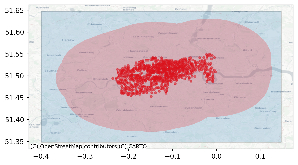
With a study area adequately encompassing the proposed reachable area, proceed to the transport routing.
Routability
As we have created a point plane naive to the transport network, it is important to check that the points are reachable by bike. Any point falling within an inaccessible portion of the transport network will report a null travel time. r5py comes with a utility function that helps to ‘snap’ unreachable locations to the nearest feature of the travel network.
Exercise 6
Part 1
Using the r5py quickstart documentation, instantiate a transport_network object, passing osm_pth as its single argument.
Part 2
- Now using the r5py advanced use section, create a new column in the
point_planegdf calledsnapped_geometry. - Use the correct method of the
transport_networkto adjust the existing geometry column. - Use a maximum search radius of 500 metres and specify the bicycle modality. Inspect the resulting geodataframe.
Part 3
Now that we have a point plane with a routable geography, we can check to ensure that the maximum search radius was observed.
- Calculate the haversine distance in metres between the original
geometryand thesnapped_geometrycoordinates. - Assign the result to
point_plane["snap_dist_m"]. - Inspect the distribution of the
snap_dist_mcolumn. Confirm that there are no values above the maximum search radius value.
Click to expand hint
Part 1
- r5py is imported as r5py. You can inspect the available classes by using the
dir()function.
Part 2
- Use
dir()on thetransport_networkobject instantiated in part 1 to find the appropriate method for snapping the coordinates to the nearest network feature. - Specify the
radiusargument with an appropriate value. - For the
street_modeargument, select the appropriate r5py transport mode. To find this value, usedir(r5py.TransportMode).
Part 3
- The
haversinefunction is imported. Unfortunately, it expects coordinates to be in a latitude, longitude order. - Apply a
lambdafunction across every row in thepoint_planeGeoDataFrame. You will need to specifyaxis=1to achieve this. - Within the lambda function, calculate the haversine distance in metres between the original coordinates and the
snapped_geometrycoordinates. Assign the output to the correctly named column. - Inspect the distribution of the haversine distances in whichever way you feel. Can you confirm that no coordinate was adjusted beyond the maximum search radius used when you instantiated the
snapped_geometrycolumn?
Solution
Part 1
Show the code
transport_network = r5py.TransportNetwork(osm_pth)This may seem like a small step, but if this passed, then you have correctly configured your Java Virtual Machine.
Part 2
Show the code
point_plane["snapped_geometry"] = transport_network.snap_to_network(
    point_plane["geometry"],
    radius=500,
    street_mode=r5py.TransportMode.BICYCLE,
)
point_plane.head()| geometry | id | snapped_geometry | |
|---|---|---|---|
| 0 | POINT (-0.40000 51.35000) | 0 | POINT (-0.40010 51.34960) |
| 1 | POINT (-0.39463 51.34995) | 1 | POINT (-0.39420 51.34960) |
| 2 | POINT (-0.38926 51.34990) | 2 | POINT (-0.38927 51.35027) |
| 3 | POINT (-0.38390 51.34985) | 3 | POINT (-0.38468 51.35024) |
| 4 | POINT (-0.37853 51.34980) | 4 | POINT (-0.37851 51.34984) |
Part 3
Show the code
# reverse the lonlat to latlon
point_plane["snap_dist_m"] = point_plane.apply(
    lambda row:haversine(
        (row["geometry"].y, row["geometry"].x),
        (row["snapped_geometry"].y, row["snapped_geometry"].x),
        unit=Unit.METERS), axis=1)

point_plane["snap_dist_m"].plot.hist(
    bins=100,
    title="Distribution of coordinate snap distance in point plane (m)"
    )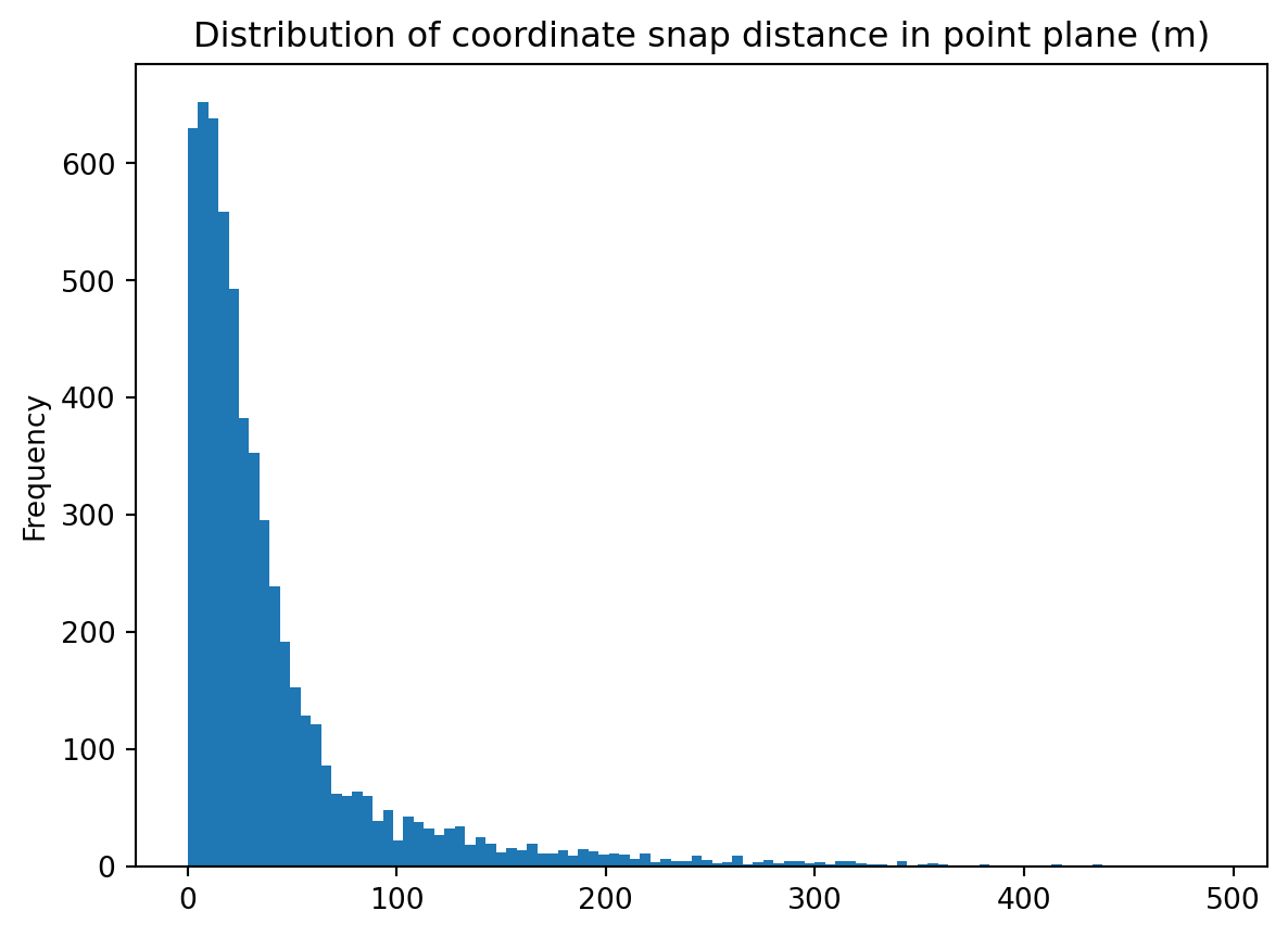
Here we can confirm that the distribution of the haversine distances is strongly right-skewed. There appear to be no values greater than 450 metres.
point_plane["snap_dist_m"].describe()count 5871.000000
mean 42.857620
std 56.671823
min 0.013986
25% 11.194528
50% 24.091469
75% 48.486417
max 491.635701
Name: snap_dist_m, dtype: float64In describing the column we can observe the actual maximum haversine distance of 492 metres. Note the differences in the mean and median are attributable to the strong skew in the distance distribution.
The spatial adjustment caused by the snapping can be visualised. This is useful for sanity-checking and edge-case investigation.
Exercise 7
Part 1
- Create a deep copy of the
point_planegeodataframe and assign to a new object calledlargest_snaps. - Retrieve the rows with the largest 100
snap_dist_mvalues. Visualising the points is expensive, so we will only display a subset. - Apply a lambda function over
largest_snaps, creating aLineStringbetween eachgeometryandsnapped_geometryvalue. This will be used to draw a line between each point on a map. - Assign the output to
largest_snaps["lines"]. - Inspect the head of the resultant geodataframe.
Part 2
- Plot
largest_snapson afoliummap. Add a marker layer with red icons showing the locations of the original point plane geometry. - Add a second marker layer to the same
foliummap, adding the snapped geometry with a green marker. - Add the final layer to the map - the lines connecting the geometries to their snapped equivalents.
- Show the map.
Click to expand hint
Part 1
- Sort ascending the
largest_snapsgeodataframe bysnap_dist_m. Take the top 100 records only. LineStringtakes 2 arguments, a start and end point coordinate.- Apply the
LineStringlogic over each row in the geodataframe, ensuring theaxisargument is set to 1. - For each row, pass the
geometrycolumn value toLineStringas the first argument, and thesnapped_geometryvalue as the second. - Assign the returned value to an appropriately named column.
Part 2
This exercise will exploit the kwargs available through the GeoDataFrame.explore() method. Alternatively, the map can be built from scratch using the folium library.
- Call explore on
largest_snaps, specifying a “marker”marker_type. Use themarker_kwdsparameter to pass a dictionary specifying which font-awesome icon to use for the geometry points. Assign the map toimap. - Set the geometry to the
snapped_geometrycolumn and repeat the above process, this time specifying green markers for the points. Ensure themparameter is set toimapin order to add this to the same map object. - Lastly, set the geometry to the
linescolumn and explore, again settingm=imapto add the line geometries to the interactive map. Specify an appropriate zoom level. - Show the map and explore the adjusted geometries.
Solution
Part 1
Show the code
largest_snaps = point_plane.copy(deep=True)
# retrieve the top 100 rows where coordinates adjusted by the greatest dist.
largest_snaps = largest_snaps.sort_values(
    by="snap_dist_m", ascending=False).head(100)
# create the LineString geometry
largest_snaps["lines"] = largest_snaps.apply(
    lambda row: LineString([row["geometry"], row["snapped_geometry"]]),
    axis=1
)
largest_snaps.head()| geometry | id | snapped_geometry | snap_dist_m | lines | |
|---|---|---|---|---|---|
| 825 | POINT (-0.39423 51.39259) | 825 | POINT (-0.39746 51.39652) | 491.635701 | LINESTRING (-0.39423 51.39259, -0.39746 51.39652) |
| 5388 | POINT (-0.22671 51.62509) | 5388 | POINT (-0.22553 51.62089) | 473.637347 | LINESTRING (-0.22671 51.62509, -0.22553 51.62089) |
| 5557 | POINT (0.12522 51.62996) | 5557 | POINT (0.11988 51.62753) | 457.484858 | LINESTRING (0.12522 51.62996, 0.11988 51.62753) |
| 5839 | POINT (-0.01873 51.64566) | 5839 | POINT (-0.02477 51.64732) | 455.327799 | LINESTRING (-0.01873 51.64566, -0.02477 51.64732) |
| 5632 | POINT (-0.02407 51.63508) | 5632 | POINT (-0.03049 51.63476) | 444.667055 | LINESTRING (-0.02407 51.63508, -0.03049 51.63476) |
Part 2
Show the code
# layer 1
z_start = 9
imap = largest_snaps.explore(
    marker_type="marker",
    marker_kwds={
        "icon": folium.map.Icon(color="red", icon="ban", prefix="fa"),
    },
    map_kwds={
        "center": {"lat": 51.550, "lng": -0.070}
    },
    zoom_start=z_start,
)
# layer 2
imap = largest_snaps.set_geometry("snapped_geometry").explore(
    m=imap,
    marker_type="marker",
    marker_kwds={
        "icon": folium.map.Icon(color="green", icon="bicycle", prefix="fa"),
    }
)
# layer 3
imap = largest_snaps.set_geometry("lines").explore(
    m=imap,
    zoom_start=z_start
)
imap
Make this Notebook Trusted to load map: File -> Trust Notebook
Travel Times
Now that we have everything we need to carry out the transport routing, there is one final adjustment to the point plane - ensure that the snapped geometries are set as the geometry column. The snapped distance and original geometry column can be removed.
point_plane.drop(columns=["geometry", "snap_dist_m"], axis=1, inplace=True)
point_plane.rename(columns={"snapped_geometry": "geometry"}, inplace=True)
point_plane.set_geometry("geometry", inplace=True)
point_plane.head()| id | geometry | |
|---|---|---|
| 0 | 0 | POINT (-0.40010 51.34960) |
| 1 | 1 | POINT (-0.39420 51.34960) |
| 2 | 2 | POINT (-0.38927 51.35027) |
| 3 | 3 | POINT (-0.38468 51.35024) |
| 4 | 4 | POINT (-0.37851 51.34984) |
Compute the Travel Time Matrix
Now we use r5py to compute the travel times from the station locations to the adjusted point plane.
Some notes on the parameters:
transport_modestakes a list of modes. For simplicity, onlyBICYCLEis used, though combining withWALKwould allow routing through portions of the travel network tagged as pedestrian-only.departure_timetakes adatetimethat signifies the first trip start time and date. This should ideally match the date that you ingested the osm file, as the osm files will best represent the real-world state of the transport network.departure_time_windowcreates a time window to carry out routing operations. The first journey occurs at 8am, as specified bydeparture. Then r5py processes a journey at every minute until thedeparture_time_windowis met. By default, r5py returns the median travel time across these journeys. This feature provides stable statistics, particularly when working with bus or train timetable data.- The points can be snapped during the computation job, by specifying
snap_to_network=True. As we have already specified how to do this, we can set this to False. max_timetakes a timedelta object. Here we specify that the journeys should take no longer than 30 minutes, as this is the current hire charge period for the bikes.- The
compute_travel_timesmethod returns a pandas DataFrame of median travel times for every origin, destination combination.
This step can be expensive, depending on the size of your point plane. Don’t be alarmed by NaN in the travel_time column. These are points in the point plane that were not reachable from any bike station.
dept_time = datetime.now().replace(hour=8, minute=0, second=0, microsecond=0)

travel_time_matrix = r5py.TravelTimeMatrixComputer(
    transport_network,
    origins=station_gdf,
    destinations=point_plane,
    transport_modes=[r5py.TransportMode.BICYCLE],
    departure=dept_time,
    departure_time_window=timedelta(minutes=10),
    snap_to_network=False,
    max_time=timedelta(minutes=30),
).compute_travel_times()

travel_time_matrix.dropna().head()| from_id | to_id | travel_time | |
|---|---|---|---|
| 2938 | BikePoints_1 | 2938 | 29.0 |
| 2939 | BikePoints_1 | 2939 | 28.0 |
| 3038 | BikePoints_1 | 3038 | 29.0 |
| 3039 | BikePoints_1 | 3039 | 29.0 |
| 3040 | BikePoints_1 | 3040 | 30.0 |
Feature Engineering
In order to produce some informative visuals, the travel time matrix will need some summarisation and feature engineering.
Exercise 8
Produce a table called med_tts with the following spec:
id                       int64
geometry              geometry
median_tt              float64
n_stations_serving       int16
n_stations_norm        float64
inverted_med_tt        float64
listed_geom             object
Part 1
- Calculate the median travel time for every point in the point plane across the stations, call the column
median_tt. - Calculate the number of bike stations that can reach each point in the point plane. Ensure that this column is formatted as “int16” and is called
n_stations_serving. - Join the medians and number of stations to
point_planeonto_id.
Part 2
- Use a minmax scaler to scale the number of stations serving each point in the point plane. Assign this to
med_tts["n_stations_norm"]. - Calculate inverteded values for the median travel time. Use the same scaling as the previous step and assign to
med_tts["inverted_med_tt"]. - Create a column with a list of the coordinate for each row, in
[long, lat]order. This is the geometry format expected by pydeck. Assign this tomed_tts["listed_geom"].
Click to expand hint
Part 1
- To create the median travel times across bike stations, group by the
to_idcolumn and calculate themedian. - To get the number of stations reaching each point, group by the
to_idcolumn and count the number offrom_idvalues. - Join the above grouped dataframes to the point plane dataframe, using the
to_idcolumn as the search key. Ensure the columns are named as specified in the exercise. - Cast
n_stations_servingto int16. First, ensure that NaNs get encoded as 0. To do this, create a boolean mask where that column is na and assign the column values that meet that boolean index to 0. Then casting to int will be possible.
Part 2
- Instantiate a
min_max_scalerusing an appropriate class fromsklearn. - Reshape the values of
n_stations_servinginto a 2D numpy array, containing enough rows for each value. - Using the
min_max_scaler, transform the numpy array. - Flatten the output of
min_max_scalerand assign to a column calledn_stations_norm. - Create a new column
inverted_med_tt, which subtracts allmedian_ttvalues from the maximum value in that column. - Scale
inverted_med_ttby repeating steps 2 through 4 for this column. - Use a list comprehension to extract each of the
geometrycoordinate values as a long,lat list. Assign tolisted_geom.
Solution
Show the code
def get_median_tts_for_all_stations(
    tt: pd.DataFrame, pp: gpd.GeoDataFrame
) -> gpd.GeoDataFrame:
    """Join travel times point geometries & calculate medians.

    Parameters
    ----------
    tt : pd.DataFrame
        Matrix of travel times where `from_id` are stations and `to_id` are
        points in the point plane.
    pp : gpd.GeoDataFrame
        Locations in the point plane.

    Returns
    -------
    gpd.GeoDataFrame
        Point plane locations with median travel times from stations and number
        of stations serving each point.

    """
    #----- Part 1 -----
    # get median travel time from all stations:
    med_tts = tt.groupby("to_id")["travel_time"].median()
    # get number of stations serving each point in the grid
    tt_dropna = tt.dropna()
    n_stations = tt_dropna.groupby("to_id")["from_id"].count()
    df = pp.join(med_tts).join(n_stations)
    df = df.rename(
        columns={"travel_time": "median_tt", "from_id": "n_stations_serving"}
    )
    # need integer for n_stations_serving but there are NaNs
    bool_ind = df["n_stations_serving"].isna()
    df.loc[bool_ind, "n_stations_serving"] = 0.0
    df["n_stations_serving"] = df["n_stations_serving"].astype("int16")
    #----- Part 2 -----
    min_max_scaler = preprocessing.MinMaxScaler()
    x = df["n_stations_serving"].values.reshape(-1, 1)
    x_scaled = min_max_scaler.fit_transform(x)
    df["n_stations_norm"] = pd.Series(x_scaled.flatten())
    max_tt = max(df["median_tt"].dropna())
    df["inverted_med_tt"] = (max_tt - df["median_tt"])
    x = df["inverted_med_tt"].values.reshape(-1, 1)
    x_scaled = min_max_scaler.fit_transform(x)
    df["inverted_med_tt"] = pd.Series(x_scaled.flatten())
    out_gdf = gpd.GeoDataFrame(df, crs=4326)
    out_gdf["listed_geom"] = [[c.x, c.y] for c in out_gdf["geometry"]]

    return out_gdf


med_tts = get_median_tts_for_all_stations(travel_time_matrix, point_plane)
med_tts.dropna().head()| id | geometry | median_tt | n_stations_serving | n_stations_norm | inverted_med_tt | listed_geom | |
|---|---|---|---|---|---|---|---|
| 1386 | 1386 | POINT (-0.14795 51.41766) | 30.0 | 1 | 0.002660 | 0.117647 | [-0.1479481, 51.4176588] |
| 1388 | 1388 | POINT (-0.13660 51.41752) | 29.0 | 1 | 0.002660 | 0.176471 | [-0.1366036, 51.4175184] |
| 1469 | 1469 | POINT (-0.25464 51.42343) | 31.0 | 1 | 0.002660 | 0.058824 | [-0.2546385, 51.4234283] |
| 1470 | 1470 | POINT (-0.25322 51.42198) | 32.0 | 2 | 0.005319 | 0.000000 | [-0.2532204, 51.4219807] |
| 1472 | 1472 | POINT (-0.23869 51.42585) | 27.5 | 2 | 0.005319 | 0.264706 | [-0.2386902, 51.4258517] |
As this final GeoDataFrame is all that is required for the remaining tutorial, go ahead and tidy up the environment.
# Tidy up
tmp.cleanup() # only needed if tmp directory used
del [station_gdf, travel_time_matrix, point_plane, transport_network, imap,
largest_snaps, z_start]
Visualise Travel Time
Exercise 9
Using the pydeck scatterplot layer docs, write a function that will take the med_tts GeoDataFrame and plot an interactive map. Use the features available in med_tts to customise the point radius and colour. Use the function to render an interactive map.
Show the code
def make_scatter_deck(
    gdf: gpd.GeoDataFrame,
    radius="(n_stations_norm * 20) + 20",
    start_lon: float=-0.005,
    start_lat: float=51.518,
    start_zoom: Union[int, float]=10,
) -> pdk.Deck:
    """Render a scatterPlotLayer of travel time & number of stations serving.

    Intended for use with output of ./src/tt-london-bikes.py ->
    ./data/interim/median_travel_times.pkl.

    Parameters
    ----------
    gdf : gpd.GeoDataFrame
        Table of grid locations and travel time from station locations.
    radius : str, optional
        A valid pydeck get_radius expression, by default
        "(n_stations_norm * 25) + 20"
    start_lon: float, optional
        The starting view longitude, by default -0.110.
    start_lat: float, optional
        The starting view latitude, by default 51.518.
    start_zoom: Union[int, float], optional
        The starting view zoom, by default 10.

    Returns
    -------
    pdk.Deck
        A rendered interactive map.

    """
    # some basic defensive checks
    if not isinstance(gdf, gpd.GeoDataFrame):
        raise TypeError(f"gdf expected gpd.GeoDataFrame, found {type(gdf)}")
    expected_cols = [
        "n_stations_serving",
        "listed_geom",
        "inverted_med_tt",
        "median_tt",
    ]
    coldiff = sorted(list(set(expected_cols).difference(gdf.columns)))
    if coldiff:
        raise AttributeError(f"Required column names are absent: {coldiff}")
    gdf = gdf.rename(columns={"n_stations_serving": "n_stats"})
    # create deck layers
    layer = pdk.Layer(
        "ScatterplotLayer",
        gdf,
        pickable=True,
        opacity=0.2,
        stroked=True,
        filled=True,
        radius_scale=6,
        radius_min_pixels=1,
        radius_max_pixels=100,
        line_width_min_pixels=1,
        get_position="listed_geom",
        get_radius=radius,
        get_fill_color="[255,(median_tt * 255), (inverted_med_tt * 255)]",
        get_line_color="[255,(median_tt * 255), (inverted_med_tt * 255)]",
    )
    # Set the viewport location
    view_state = pdk.ViewState(
        longitude=start_lon,
        latitude=start_lat,
        zoom=start_zoom,
        min_zoom=5,
        max_zoom=15,
        pitch=40.5,
        bearing=-27.36,
    )
    tooltip = {
        "text": "Stations serving: {n_stats}\nMdn travel time: {median_tt}"
    }
    # Render
    r = pdk.Deck(
        layers=[layer], initial_view_state=view_state, tooltip=tooltip
    )
    return r


r = make_scatter_deck(med_tts)
r
Take some time to study the map. Pan in and out by scrolling. The angle of the map can be adjusted by shift + clicking and dragging the mouse left to right. Find the point with the greatest number of stations serving. Look for any curious patterns in the median travel time. Take a look at the Greenwich peninsula, where the River Thames appears to limit accessibility from the North.
Exercise 10
Lastly, we can identify those points within the thirty minute reachable area from the bike station network that are the most remote. Let’s visualise the 20 most remote locations. These would represent candidate locations for increasing the coverage of the bike network within the thirty minute reachable zone. Once more, please note that the point grid is naive to locations where people live or would like to travel to and from.
Click to expand hint
- Sort descending the
med_ttdataframe onmedian_ttandn_stations_serving. - Take the top 20 records.
- Pass this dataframe to the function you wrote in exercise 9.
Show the code
n_isolated = (
    med_tts.dropna()
    .sort_values(["median_tt", "n_stations_serving"], ascending=[False, False])
    .head(20)
)
r = make_scatter_deck(n_isolated, radius=50, start_zoom=9.5)
r
Tips
- Most of the packages used in this tutorial expect the sequence of coordinates to be long, lat. If you select an alternative method for mapping visuals, remember to check that this is consistent. If you are getting empty interactive map visuals, pan out and check if an incorrect coordinate specification has resulted in your points being rendered off the East coast of Africa.
- The exception to the above rule is
haversine, which expects lat, long.
Conclusion
If you made it this far, well done! This tutorial has got you up and running with the r5py package. You have used several libraries in the python GIS stack to execute an analysis of bike station locations in London:
- Station locations were ingested with TfL’s api.
- OpenStreetMap data was ingested from the BBBikes download service.
- A point plane of your size was generated.
- The coverage of the point plane was inspected.
- The point plane features were adjusted to the underlying transport network.
- Median travel times from bike stations to the point plane were calculated.
- Travel times were summarised and features engineered for presentation in informative
pydeckmaps.
Next steps for this work would be to explore how potential station locations could be informed by places where people would wish to commute, such as retail, businesses, tourist attractions and residential areas. OpenStreetMap files are a rich source of location data, which can be extracted with libraries such as pyosmium.
Service optimisation is an interesting area of operational research. This analysis does not consider local demand on the stations and their capacity to meet that demand. This sort of problem is known as the capacitated facility location problem and can provide operational efficiencies while improving service quality for the customer.
fin!
References
[1]
“r5py Installation documentation.” https://r5py.readthedocs.io/en/stable/user-guide/installation/installation.html
[2]
“EC Global Human Settlement Layer.” https://ghsl.jrc.ec.europa.eu/download.php
[3]
“Santander Cycles - What you pay.” https://tfl.gov.uk/modes/cycling/santander-cycles/what-you-pay
[4]
I. Yamada, “Edge Effects,” International Encyclopedia of Human Geography, pp. 381–388, 2009.